Which endothelial genes are enriched under murine sepsis treatment?

My lab is interested in endothelial cells. My interest in particular is the role of endothelial cells in the pathophysiology of sepsis.

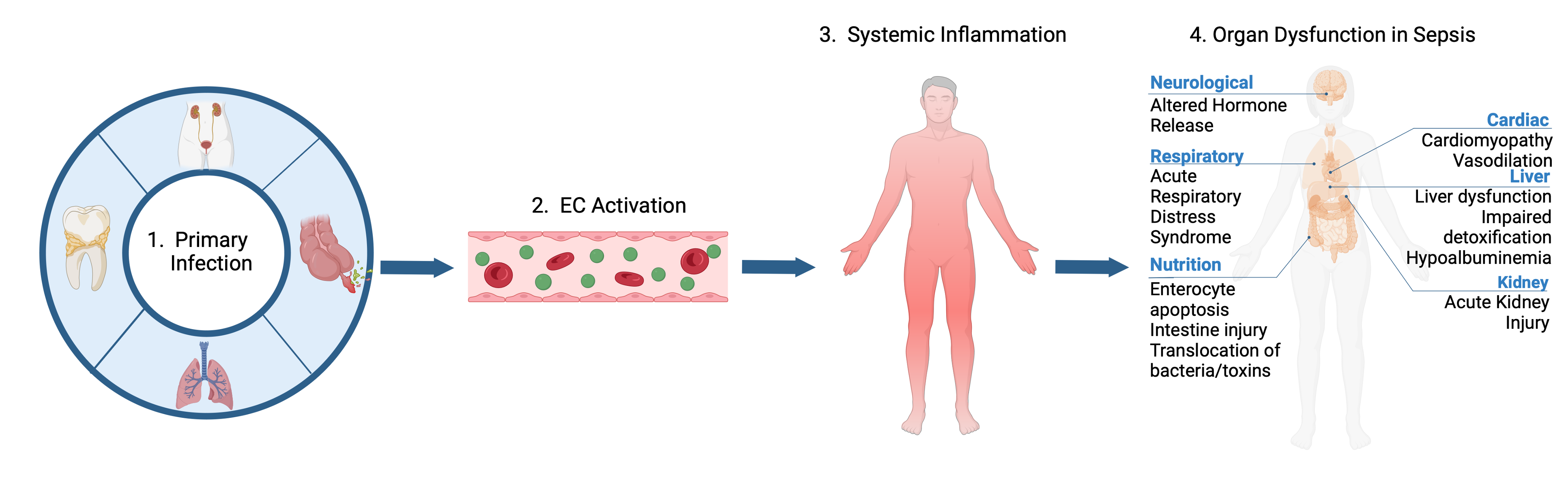
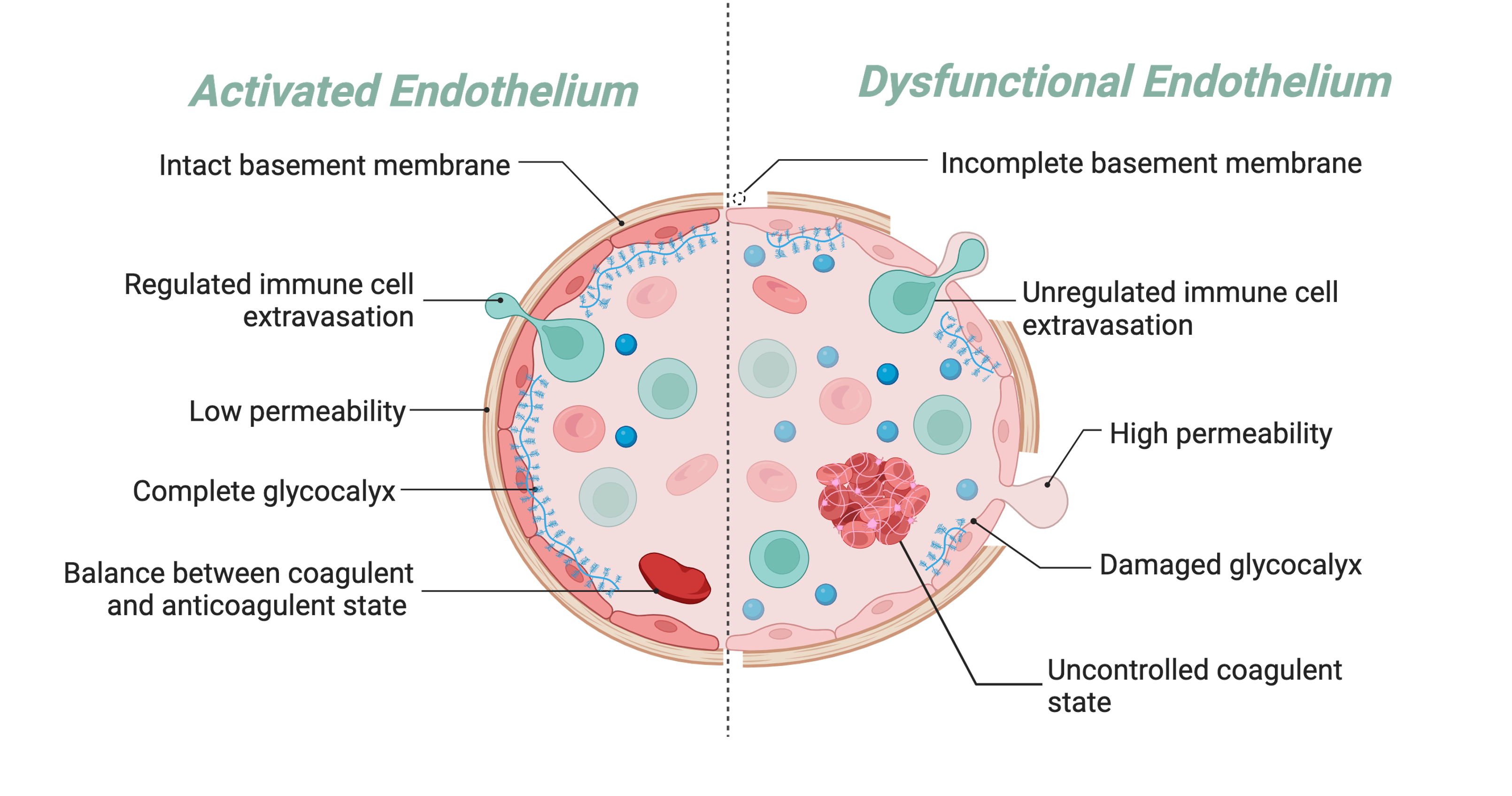
Sepsis begins as a primary infection. Like any other infection, endothelial cells (ECs) are a part of your first responders that directly and indirectly respond to pathogens. To that end, endothelial cells become activated where they undergo phenotypic changes to better attack a pathogen. These changes include increasing their vascular permeability for leukocytes to extravasate into the tissue to help fight the pathogen. ECs with also increase their inflammatory response by secreting cytokines to further recruit an immune response. Lastly, ECs will switch to a more procoagulant state so they can trap the pathogen from entering circulation.

As a pathogen persists in cases like sepsis, the phenotypic changes that were once helpful in clearing the pathogen become detrimental to the host as the ECs are unable to return to quiescence. The increased vascular permeability gives rise to the vascular leakage driving organ dysfunction in sepsis complications.

In order to look at endothelial cells specifically, I am using a Cdh5-driven inducible Cre to produce a hemagglutinin tagged ribosomal protein 22. By tissue harvest, followed by immunoprecipitation of the hemaglutein tagged polyribosomes, I can capture the actively translated mRNA from endothelial cells and determine which transcripts are enriched or depleted in endothelial cells.

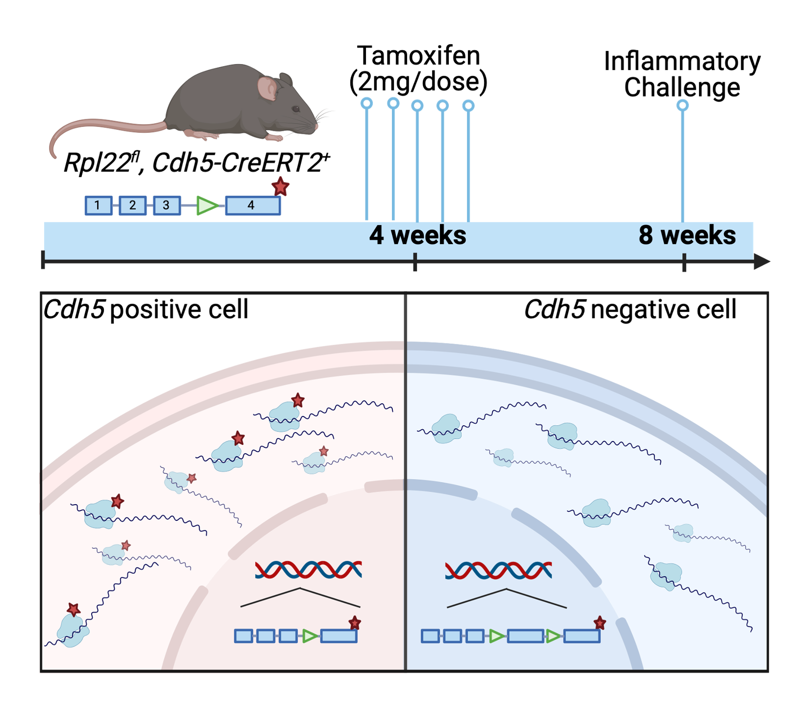
Because I am particularly interested in sepsis-induced acute kidney injury, I began with RNA Seq data from renal mRNA of control and sepsis-treated mice.

Step 1: Load required libraries and data set to be analyzed

library(dplyr)
library(ggplot2)
library(tidyverse)

df <- read.table("FSIvsControlBead.csv", sep = ',')

Step 2: Rename columns in R for simplicity

df <- read.csv("FSIvsControlBead.csv", header = TRUE, check.names = TRUE)

colnames(df)

[1] "X"                            "symbol"                      
[3] "B_FSI_vs_Ctrl_baseMean"       "B_FSI_vs_Ctrl_log2FoldChange"
[5] "B_FSI_vs_Ctrl_pvalue"         "B_FSI_vs_Ctrl_padj"

names(df)[names(df) == "B_FSI_vs_Ctrl_padj"] <- "padj"

names(df)[names(df) == "B_FSI_vs_Ctrl_log2FoldChange"] <- "FC"

print(names(df))

[1] "X"                      "symbol"                 "B_FSI_vs_Ctrl_baseMean"
[4] "FC"                     "B_FSI_vs_Ctrl_pvalue"   "padj"

Step 3: Set appropriate threshold for data of interest

fc_threshold <- 1
padj_threshold <- 0.05

padj <- padj_threshold
FC <- fc_threshold

Step 4: Define significant genes

sig_genes <- df |> 
  filter(!is.na(padj)) |> 
  filter(padj <= padj_threshold & abs(FC) >= fc_threshold)

df <-df |>
mutate(significant = ifelse(!is.na(padj) & padj < padj_threshold & abs (FC) > fc_threshold, "yes", "no"))

Step 5: Create Volcano Plot

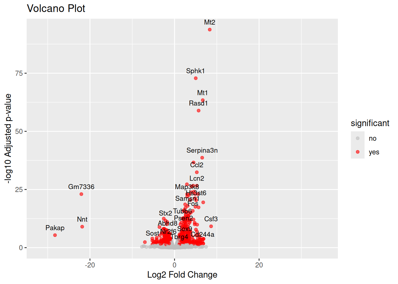
ggplot(df, aes(x = FC, y = -log10(padj), label = symbol)) +
  geom_point(aes(color = significant), alpha = 0.6) + 
  scale_color_manual(values = c("yes" = "red", "no" = "gray")) +
  labs(
    title = "Volcano Plot",
    x = "Log2 Fold Change",
    y = "-log10 Adjusted p-value"
  ) +
  geom_text(
    data = subset(df, significant == "yes"),
    vjust = -1,
    size = 3,
    check_overlap = TRUE
  )

Step 6: Create Top Genes List

top_genes <- sig_genes %>%
arrange(desc(abs(FC))) %>%
slice(1:10)

top_genes

                    X  symbol B_FSI_vs_Ctrl_baseMean         FC
1  ENSMUSG00000089945   Pakap               5.443726 -28.276875
2  ENSMUSG00000078636  Gm7336             106.543665 -22.042611
3  ENSMUSG00000116207     Nnt             179.256057 -21.841981
4  ENSMUSG00000038067    Csf3            1161.682682   8.645900
5  ENSMUSG00000031762     Mt2           21591.364410   8.327600
6  ENSMUSG00000058743  Kcnj14               7.970885  -7.009475
7  ENSMUSG00000062061   Obp2a               9.716260   6.875721
8  ENSMUSG00000026073   Il1r2              20.287552   6.800744
9  ENSMUSG00000058427   Cxcl2            1607.268006   6.786794
10 ENSMUSG00000019368 Sec14l4              43.355829   6.786016
   B_FSI_vs_Ctrl_pvalue         padj
1           3.68000e-08 4.320000e-06
2           9.72000e-27 9.900000e-24
3           4.53000e-12 9.970000e-10
4           2.95000e-12 6.780000e-10
5           1.13000e-98 1.830000e-94
6           1.44936e-04 4.233525e-03
7           2.93000e-06 1.767510e-04
8           2.32000e-06 1.473960e-04
9           4.79000e-23 3.400000e-20
10          9.14820e-04 1.807352e-02

ggplot(top_genes, aes(x = reorder(symbol, FC), y = FC, fill = FC > 0)) + 
  geom_col() + 
  coord_flip() + 
  labs(title = "Top 10 Most Affected Genes", 
       x = "Gene", 
       y = "Log2 Fold Change") + 
  scale_fill_manual(name = "Direction", 
                    values = c("TRUE" = "steelblue", "FALSE" = "salmon"), 
                    labels = c("FALSE" = "Downregulated", "TRUE" = "Upregulated")) + 
  theme_minimal()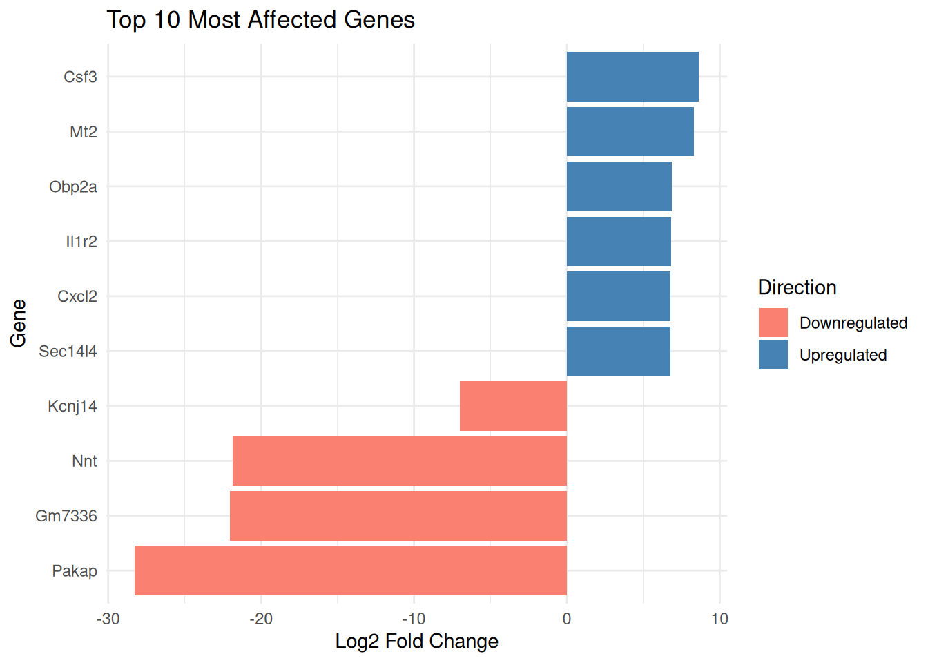

This analysis gives me a better idea of what genes or pathways are potentially contributing to the pathology of sepsis-induced acute kidney injury, and I can use these genes as a guide in the future to determine if a therapeutic option had a beneficial effect.